![]()
8 Puzzle Algorithm
8 puzzle is a very interesting problem for software developers around the world. It always has been an important subject in articles, books and become a part of course material in many universities. It is a well known problem especially in the field of Artificial Intelligence. This page is designed to tell you the very basic understanding of the algorithm to solve the 8 puzzle problem. You may find "what the problem is" from the 8 puzzle problem page If you still don't have any idea about it.
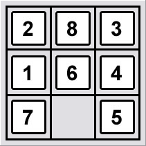
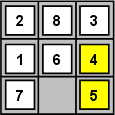
As it's mentioned in the 8 puzzle problem page, the game has an initial state and the objective is to reach to the goal state from the given initial state. An example initial state and corresponding goal state is shown below.
 |
 |
| Initial State | Goal State |
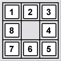
Before beginning to tell how to reach from the initial state to the goal state, we have to solve a sub problem which is "choosing the goal state to be reached". As it's mentioned in the 8 puzzle problem page, the game has two possible arrangements. We have to choose one of the goal states to be reached because only one of them is reachable from the given initial state. Sounds interesting? Lets see why the 8-puzzle states are divided into two disjoint sets, such that no state in one set can be transformed into a state in the other set by any number of moves.
|
|
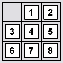 |
| Goal State A | Goal State B |
First we begin with the definition of the order of counting from the upper left corner to the lower right corner as shown in the figure below.
 |
| Order of Counting |
This definition is given because we need to determine the number of smaller digits which are coming after a chosen tile. Its a little bit trick to tell with words. So lets have an example.
 |
| Counting Example 1 |
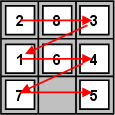
In this example above we see the tiles which comes right after tile #8 and smaller than 8, in yellow. So if we count the yellow tiles, we get 6. We will apply this counting for every tile in the board. But first lets have another example to make things crystal clear.
 |
| Counting Example 2 |
This time we count the tiles which comes right after tile #6 and smaller than 6, in yellow. As a result we get 2. Now we made things clear on how to count. Now we will do this counting for every tile in the board.
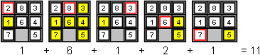 |
| Counting the Board |
In the figure below you see that counting for tile #1 is skipped. That's because the result is always 0 (1 is the smallest tile). Counting for each tile has been done and then the results are summed. Finally we get 11 as the result.
Now I believe that most of you have the question "So, what?". The answer is simple. As you can imagine the result is always either even or odd. And this will be the key to solve the problem of "choosing the goal state to be reached". Lets call the result as N.
If N is odd we can only reach to the Goal State A as shown below. If N is even we can only reach to the Goal State B as shown below.
|
|
|
| Goal State A | Goal State B |
Of course this is not an arbitrary selection. There is a logic behind it and here is the proof. First, sliding the blank along a row does not change the row number and not the internal order of the tiles, i.e. N (and thus also Nmod2) is conserved. Second, sliding the blank between rows does not change Nmod2 either. You can try these things on paper and understand the idea behind it more clearly.
Now we have determined which goal state to reach, so we can start a search. The search will be an uninformed search which means searching for the goal without knowing in which direction it is. We have 3 choices for the search algorithm in this case. These are:
- Breadth-first search algorithm
- Depth-first search algorithm
- Iterative deepening search algorithm
When we chose any of this algorithms to apply, we will start with the initial state as the beginning node and search the possible movements of the blank. Each time we move the blank to another position (create a new board a arrangement) we create a new node. If the node we have is the same as goal state then we finish the search.
The three algorithms given above differs on the choice of the search path (node to node). Below you will find summarized descriptions
Breadth-first search algorithm: finds the solution that is closest (in the graph) to the start node that means it always expands the shallowest node. See Wikipedia for more information
Depth-first search algorithm: starts at the root (selecting some node as the root in the graph case) and explores as far as possible along each branch before backtracking.
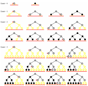 |
| Iterative Deepening Search Image from Russell and Norvig, Artificial Intelligence Modern Approach, 2003 |
Iterative deepening search algorithm: is a modified version of the dept first search algorithm. It can be very hard to determine an optimum limit (maximum depth) for depth first search algorithm. That's why we use iteration starting from the minimum expected depth and search until the goal state or the maximum depth limit of the iteration has been reached. See Wikipedia for more information
Because of its properties we will use iterative deepening search algorithm.